
This post details my contribution for a final group project in CSE 842 - Natural Language Processing at Michigan State University. My group members were Luke Sperling and Xavier Williams.
Estimating a text’s readability is useful for many reasons! Educators want to know what books are appropriate for their students, authors want to know what reading level their writing fits with to accommodate their target audience, etc. Readability is an arbitrary score which attempts to create a scale to help readers gauge the difficulty a reader might have when encountering a text.
There is no ground truth for readability. It is determined by some function of the input text features. Several metrics have been introduced, such as the Flesch-Kincaid Scale, the Automated Readability Index, and others. Many of these are available to anyone through the PyPI readability package, and use some function of word frequency (as a proxy for semantic complexity) and and sentence length (as a proxy for syntactic complexity).
Lexile is a very popular example of these frameworks. Developed by MetaMetrics, the Lexile System (LS) scores text according to the following: first, the text is split into 80-word slices which are compared against the 600-million word Lexile corpus. Next, the word frequency and sentence length are extracted and input to the proprietary Lexile equation. The output of the equation is then applied to the Rasch psychometric model to determine the Lexile measure for the text as a whole.1
Unfortunately, the Lexile framework is proprietary and not open-source, which makes it more difficult for new authors to get Lexile scores or for educators to get scores of books not in the database. Let’s test how well these scores can be reverse engineered by training a neural net on a dataset of books and their scores!
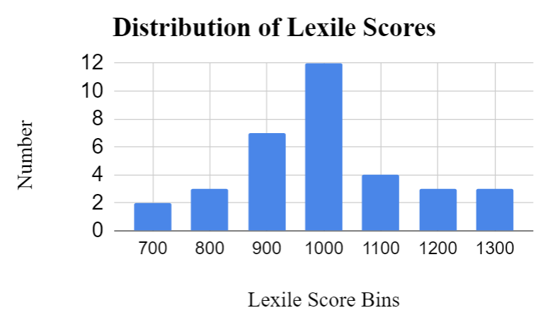
The dataset I’ll be using had to be built using public domain books from Project Gutenberg, which means my dataset is very small compared to the one lexile uses, but there are enough texts to represent each class that I plan to predict. Lexile scores range from 200 - 1700, but the majority of texts fall into 7 bins which I will be predicting in this project. Each bin represents a range of 100 in Lexile scores. The distribution of the dataset is shown below:
Preprocessing
Now that the goal is clear, let’s import the data and start preprocessing the text.
# Import data
data = []
for i in range(1, 35):
    #filename = "./Book Files/" + str(i) + ".txt"
    filename = str(i) + ".txt"
    data.append(filename)

# Define a preprocessing function
def Preprocess(data, test_size):
    #data is in the format: [filename]
    Xy = []
    lexile_converter = [700,800,900,1000,1100,1200,1300]#7 bins, value is the max of that bin
    for filename in data:
        directory = "/Users/home/CSE 842 Project NN/Book Files/" + filename
        fp = open(directory,'r', encoding="utf8")
        first_line = fp.readline().strip()#lexile measure is in this line

        index = 0
        for i, ch in enumerate(first_line):#this shears off weird formatting characters off line 1
            if ch.isdigit():
                index = i
                break
        lexile = int(first_line[index:])
        lexile_bin = 1300
        for value in lexile_converter:#find what bin our lexile measure falls into
            if lexile <= value:
                lexile_bin = value
                break
        contents = ""
        count = 0
        for line in fp:#add 100 word chunks to be used as data point
            line = line.strip()
            contents = contents + line
            count+=1
            if count==100:
                count=0
                #X.append(contents)
                #y.append(lexile_bin)
                Xy.append((contents,lexile_bin))
                contents = ""

    #shuffle up our dataset
    random.shuffle(Xy)

    """
    X_train = X[:int(len(X)*(1-test_size))]
    X_test = X[int(len(X)*(1-test_size)):]

    y_train = y[:int(len(y)*(1-test_size))]
    y_test = y[int(len(y)*(1-test_size)):]
    """
    Xy_train = Xy[:int(len(Xy)*(1-test_size))]
    Xy_test = Xy[int(len(Xy)*(1-test_size)):]

    X_train = [item[0] for item in Xy_train]
    y_train = [item[1] for item in Xy_train]

    X_test = [item[0] for item in Xy_test]
    y_test = [item[1] for item in Xy_test]


    return X_train, y_train, X_test, y_test

X_train, y_train, X_test, y_test = Preprocess(data, 1/5)
There’s 41 books total in the dataset, so this preprocessor breaks those books up into 100-word chunks, resulting in ~3,000 chunks for training and testing.
Next, I’m going to create a Pandas dataframe with the preprocessed data to further prepare it for model training.
train = pd.DataFrame(list(zip(X_train, y_train)), columns = ['Text', 'Score'])
test = pd.DataFrame(list(zip(X_test, y_test)), columns = ['Text', 'Score'])

def token_count(text):
    """function to count number of tokens"""
    length=len(text.split())
    return length

def tokenize(text):
    """tokenize the text using default space tokenizer"""
    lines=(line for line in text.split("\n") )
    tokenized=""
    for sentence in lines:
        tokenized+= " ".join(tok for tok in sentence.split())
    return tokenized

train['tokenized_text'] = train['Text'].apply(tokenize)
train['token_count'] = train['tokenized_text'].apply(token_count)

test['tokenized_text'] = test['Text'].apply(tokenize)
test['token_count'] = test['tokenized_text'].apply(token_count)

data = pd.concat([train, test])
Embedding
Now that the data is ready, it’s time to decide on an embedding. Though semantic embeddings like word2vec or a BERT approach might be appealing, it’s important that the embeddings capture similar information to the Lexile model. While it’s true that using BERT might produce reading scores that more accurately reflect the semantics of the text, the goal of this project is to recreate Lexile scores; otherwise there won’t be an appropriate metric for our model. For this case, TF-IDF is going to be the best method.
# Create TF-IDF for the text

num_max = 4000

def train_tf_idf_model(texts):
    "train tf idf model"
    tok = Tokenizer(num_words=num_max)
    tok.fit_on_texts(texts)
    return tok

def prepare_model_input(tfidf_model, dataframe, mode='tfidf'):
    "function to prepare data input features using tfidf model"
    le = LabelEncoder()
    sample_texts = list(dataframe['tokenized_text'])
    sample_texts = [' '.join(x.split()) for x in sample_texts]

    targets=list(dataframe['Score'])
    sample_target = le.fit_transform(targets)

    if mode=='tfidf':
        sample_texts=tfidf_model.texts_to_matrix(sample_texts,mode='tfidf')
    else:
        sample_texts=tfidf_model.texts_to_matrix(sample_texts)

    print('shape of labels: ', sample_target.shape)
    print('shape of data: ', sample_texts.shape)

    return sample_texts, sample_target

# Train TF-IDF
texts = list(data['tokenized_text'])
tfidf_model = train_tf_idf_model(texts)
# prepare model input data
mat_texts, tags = prepare_model_input(tfidf_model, data, mode='tfidf')
Model
Alright, let’s fire up a neural network and start classifying! For the neural net, I’ll be using the Keras framework. I found it well-suited to this problem since we’re using a small dataset and a simple feed-forward model architecture.
def get_simple_model():
    """
    Uses 3 layers: Input -> L1 : (Linear -> Relu) -> L2: (Linear -> Relu)-> (Linear -> Sigmoid)
    Layer L1 has 512 neurons with Relu activation
    Layer L2 has 256 neurons with Relu activation
    Regularization : We use dropout with probability 0.5 for L1, L2 to prevent overfitting
    Loss Function : binary cross entropy
    Optimizer : We use Adam optimizer for gradient descent estimation (faster optimization)
    Data Shuffling : Data shuffling is set to true
    Batch Size : 64
    Learning Rate = 0.001
    """
    model = Sequential()
    model.add(Dense(512, activation='relu', input_shape=(num_max,)))
    model.add(Dropout(0.5))
    model.add(Dense(256, activation='relu'))
    model.add(Dropout(0.5))
    #model.add(Dense(7, activation='softmax'))
    model.add(Dense(7,))
    model.add(Activation('softmax'))
    model.summary()
    model.compile(loss='binary_crossentropy',
              optimizer='adam',
              metrics=['acc',keras.metrics.categorical_accuracy,])
    print('compile done')
    return model

def fit_model(model,x_train,y_train,epochs=10):
    history=model.fit(x_train,y_train,batch_size=64,
                      epochs=epochs,verbose=1,
                      shuffle=True,
                      validation_split = 1/9,
                      callbacks=[checkpointer, tensorboard]).history
    return history

# define checkpointer
checkpointer = ModelCheckpoint(filepath=model_save_path,
                               verbose=1,
                               save_best_only=True)

# define tensorboard
tensorboard = TensorBoard(log_dir='./logs',
                          histogram_freq=0,
                          write_graph=True,
                          write_images=True)

# Split into training and test data
from sklearn.model_selection import train_test_split

X_train, X_val, y_rtrain, y_rval = train_test_split(mat_texts, tags, test_size=0.15)
y_train = keras.utils.to_categorical(y_rtrain)
y_val = keras.utils.to_categorical(y_rval)
y = tags

# Initialize our model
model = get_simple_model()

# Train
history=fit_model(model,X_train,y_train,epochs=10)
Results
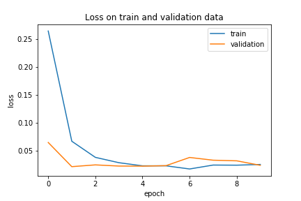
Turns out, this model has no problem learning each of the 7 bins in our data! The model picks up on the patterns early in training:
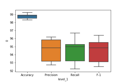
And after a 10-fold cross-validation, the model achieves 98.76% accuracy. Remember that the data was skewed towards the middle classes, so maybe there’s a lot of false positives in the results. However, the (macro) F-1 score is 94%, so the model is doing well predicting each class. Here’s the distribution of metric values for the model after cross-validation:
Conclusion
This project shows that a neural net can easily provide an alternative to authors, educators, and anyone else who doesn’t have access to the Lexile model but wants to know the Lexile score for a text. Just for fun, let’s run some new texts through the model and see what scores are predicted. (Score bins are predicted for each 100-word chunk and the final prediction is an average of each chunk’s prediction.)
| Text | Predicted Score |
|---|---|
| Book of John (KJV) | 1040 |
| Book of John (NIV) | 920 |
| US Constitution | 1200 |
| Jurafsky & Martin Chapter 4 | 980 |
The King James Version (KJV) of the Bible, which is known for its antiquated English, has a Lexile score of 1000 according to the Lexile database. This model predicts that the book of John in the KJV has a score of 1040. Not bad! A more modern translation, the New International Version (NIV) has a score of 920, which is expected given the updated English. The other texts used were the US Constitution, which the model suggests is a few levels more difficult at 1200, and a chapter of a book responsible for a lot of my NLP education, Chapter 4 of Speech and Language Processing by Daniel Jurafsky & James H. Martin2, which scored a 980.
Looking forward, it would be possible to create a model that discretizes the scores into smaller bins if the dataset was expanded. It also goes to show that even with all the hype over more recently-conceived embedding schemes, there are many NLP tasks where TF-IDF still gives great results.